Benchmark data sets for the problem dividing graphs into bi-connected components with a size constraint

Raka Jovanovic

(This is not the final version)

The generated test instances and code can be downloaded from

1. Data

2. Code

On this webpage we give test instances for the Problem of dividing graphs into bi-connected components with a size constraint. The data has been used in the article

1. A heuristic approach for dividing graphs into bi-connected components with a size constraint, Raka Jovanovic, Tatsushi Nishi, Stefan Voss, Journal of Heuristics

In case you wish to use this data please contact me by email at rakabog@yahoo.com, regarding referencing and if you need help using the data.

Problem Definition

The problem is defined on a graph , where is the set of nodes and is the set of edges. We also define a set, whose elements will be called root nodes. The aim of the problem is to divide the graph into a set of subgraphs }$, where , satisfying the constraints given in the following text. The notation will be used for the set of nodes that induces subgraph . Each of the must contain only one distinct root node . A node can be an element of at most one . The number of nodes in each of the subgraphs is less or equal to some constant . The last constraint is that each of the subgraphs is bi-connected. The goal of the problem is to find containing the maximal number of nodes in all the subgraphs. More formally, we wish to maximize the sum:

where each of the subgraphs satisfies

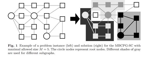
In the definition we use notation to indicate the number of nodes in a graph. An illustration of a problem instance and solution for the MBCPG-SC is given in following figure. It is important to note that the MBCPG-SC does not produce a partitioning in the strict sense, since some nodes may not be included in any .

Problem Instances

The problem instances consist of a wide range of synthetically generated problem instances for different numbers of root nodes n (5-100) and maximal allowed number of nodes in a subgraph M (5-100). For each pair (n, M) 40 problem instances have been generated using the algorithm presented in the mentioned article. Further there are we have also generated problem instances based on the power flow data from Poland, France, EU and standard IEEE benchmark problem instances. To be more precise we have used the data provided my MatPower.

The generated test instances have been made available for download.

The code for the results given in the article (under review) can also be downloaded. The source code is given as a C# project in Visual Studio together with executable files. The code is just an alpha version so it is very buggy. If you wish to use the code please contact me. For the exe to work copy the test instances to the \Work\Release folder

File Structure

Benchmark data sets are given in one zip file. The file has two folders Basic(with subfolders Alpha2 and Alpha15) for synthetically and RW for real world based problem instances.

In case of problem instance in folder Basic each one has 3 related files.

“x.pro” the problem instance

“x.sol” optimal solution for the problem

“x.vis” is an additional file giving the coordinates of the graph which can be used for visualization.

The problem instances in folder RW have the “x.pro” .

The structure of the files is intuitive, but we give the following explanation of the structure

The “pro” files have the following structure:

“Number Of Nodes” % line included for easy reading

N % number of supply nodes

“Number of Subgraphs” % line included for easy reading

S % Number of subgraphs/root nodes

“Number of nodes in subgraph” % line included for easy reading

NS % Number of demand nodes

Roots Nodes % line included for easy reading

S Lines consisting of one integer value. % each gives the Id of a rot node

Node Ids start from 0

Graphs % line included for easy reading

NumberOfVertices % line included for easy reading

NV % integer number

Edges % line included for easy reading

%For each Vertex the list of neighboring nodes is given

Number edges containting node X % line included for easy reading

NE % integer number

list % line included for easy reading

NE lines each having a node ID

The “sol” files have the following structure:

Number Of Subgraphs % line included for easy reading

S

Number Of Nodes In Subgraphs % line included for easy reading

NS

% for each subgraph

PARTITION X % line included for easy reading

Nodes Inside % line included for easy reading

NN % Number Of Nodes Inside

list % line included for easy reading

NN lines each having a node ID

The “vis” files have the following structure:

Number of Vertices % line included for easy reading

NV % integer number

Node Positions X Y % line included for easy reading

NV lines having X, Y coordinates separated with a space

The files for one problem size

In case of instances in folder Basic for each of the problem sizes there are 40 different problem instances. We have used the following file naming convection:

“prob_S_N_I.gpr”, “sol_S_N_I.Vis”, . Where “S” gives the number of subgraphs, “N” the maximal number of nodes in a subgrah and “I” the number of the instance. For example for a problem instance with 50 subgraphs nodes, and the maximal number of nodes is 5 demand nodes, the 15 problem instance files would have the following names

“prob_50_5_15.pro”, “prob_50_5_15.sol”, “prob_50_5_15.vis”.

In case of the RW folder the problem instances have the structure “x.pro” where “x” corresponds to the name of the MathPower file that has been used for generating the problem instance.