Benchmark data sets for the problem of partitioning graphs with supply and demand

Raka Jovanovic

(This is not the final version)

On this webpage we give test instances for the Problem of Partitioning Graphs with Supply and Demand. The data has been used in the article

1. A Heuristic Method for Solving the Problem of Partitioning Graphs with Supply and Demand, Raka Jovanovic, Abdelkader Bousselham, Stefan Voss, Annals of Operations Research, DOI: 10.1007/s10479-015-1930-5

2. A mixed integer program for partitioning graphs with supply and demand emphasizing sparse graphs, Raka Jovanovic, Stefan Voß, Optimziation Letters (2015), DOI: 10.1007/s11590-015-0972-6

3. An ant colony optimization algorithm for partitioning graphs with supply and demand, Raka Jovanovic, Milan Tubab, Stefan Voß, Applied Soft Computing (2016) DOI:10.1016/j.asoc.2016.01.013

And a similar test set is used in

4. A greedy method for optimizing the self-adequacy of microgrids presented as partitioning of graphs with supply and demand., Jovanovic R, Bousselham A, In: The 2nd International Renewable and Sustainable Energy Conference Ouarzazate, Morocco October 17-19, 2014, IEEE conference, pp 565 – 570

In case you wish to use this data please contact me by email at rakabog@yahoo.com, regarding referencing and if you need help using the data.

Problem Definition

This is one of the classical problems in graph theory. It is formulated as follows:

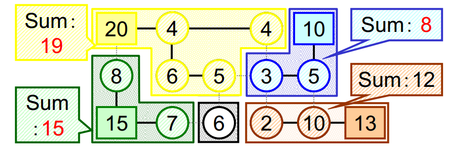
Let be an undirected graph with a set of vertices and a set of edges . is split into two disjunct sets and . Each vertex is called a supply vertex and has a corresponding positive integer value . Similarly, the vertex is called a demand vertex and has a corresponding positive integer value . Each demand vertex can receive “power” from one supply vertex through the edges of . The goal is to partition the graph into several connected subgraphs in a way that each of them has one supply vertex and demands that are less and equal to it. The goal is to maximize the fulfillment of demands, or more precisely to maximize the sum , where is the set of sub graphs.

Problem Instances

To be make it possible to have a comprehensive evaluation of algorithms for the problem of partitioning graphs with supply and demand a wide range of problem instances have been generated. Test instances graphs having 6-400 supply nodes and 6-8000 demand nodes. For each of the test sizes 40 different problem instances have been generated using different random seeds. Two types of graphs have been generated trees and general ones.

The problem instances (graphs) for n supply and m demand nodes have been generated using the following algorithm. First we would generate an array containing n+m integer random weights uniformly distributed inside of the interval [-10,-40]. In case of general graphs, (n+m)*2 random edges would be added to the graph but making sure that the graph is connected. In case of the second type of graphs case of trees we would simple generate a random tree for n+m nodes. For both type of trees, the next step was to select n random nodes as seeds for n subgraphs (partitions). The subgraphs would be grown using a iterative method until (n+m)*(0.95) nodes of the original graph are contained in one of the subgraphs. The growth of subgraph S_i has been performed by expending it to a random neighboring node that does not belong to any of the other subgraphs. Finally, for each of the subgraphs S_i a random vertex v \in S_i is chosen and its weight w is set using the following formula

w = |\sum_{a \in S_i}sup(a)| +sup(v)

For each of the test graphs, generated using this method, the best optimal solution is known and is equal to the sum of supplies of all supply nodes. It is important to mention that by using such a procedure it is possible to have partitioning that do not have n subgraphs due to some supply nodes being cut off from the rest of the graph. We have excluded such graphs from our test cases.

The generated test instances have been made available for download.

The code for the results given in the article (under review) can also be downloaded. The source code is given as a C# project in Visual Studio together with executable files. The code is just an alpha version so it is very buggy. If you wish to use the code please contact me. For the exe to work copy the test instances to the \Work\Release folder

File Structure

Benchmark data sets are given in one zip file. The file has two folders General, Tree which hold all the problem instances for the specific type of graphs.

In each of these folders there are pairs of “x.gpr” files which give a problem instance definition and “x.sol” which gives the optimal solutions for this instance. The structure of the files is intuitive, but we give the following explanation of the structure

The “gpr” files have the following structure:

“Number of Supply” % line included for easy reading

N % number of supply nodes

“Number of Demmand” % line included for easy reading

M % Number of demand nodes

Weights % line included for easy reading

N+M Lines consisting of one integer value. % Positive means supply node, negative demand node.

Node Ids start from 0

Edges % line included for easy reading

N+M Pairs of lines

Edges(I) % Indicates that edges connected to I will be given next

A line with a list on integers % list of nodes to which node %I% is connected

The “sol” files have the following structure:

Number Of Partitions ” % line included for easy reading

N % Number of Partitions

N Pairs of lines

SupplyNode I % line included for easy reading, Gives information that I is the supply node

A line with a list of integers % All these nodes are a part of the current partition

The files for on problem size

For each of the problem sizes there are 40 different problem instances. We have used the following file naming convection:

“test_S_D_I.gpr”, “sol_S_D_I.sol”. Where “S” gives the number of supply nodes, “D” the number of demand nodes and “I” the number of the instance. For example for a graph with 50 supply nodes, and 500 demand nodes, the 15 problem instance files would have the following names

“test_50_500_15.gpr”, “sol_50_500_15.gpr”.

For each number N of supply nodes we have generated graphs with (N*3, N*5, N*10, N*20) demand nodes.