Benchmark data sets for the problem of partitioning supply / demand graphs
with limited capacity
Raka
Jovanovic
(This is
not the final version)
On this webpage we give test instances for the Problem of Minimal Partitioning Supply/Demand Graphs with limited capacity (MPGSD-LC). The data has been used in the article
Partitioning of Supply/Demand Graphs with Capacity Limitations - An Ant Colony Approach, Raka Jovanovic, Abdelkader Bousselham, Stefan Voss, Journal of Combinatorial Optimization, DOI: 10.1007/s10878-015-9945-z
In case you wish to use this data please contact me by email at rakabog@yahoo.com, regarding referencing and if you need help using the data.
Problem Definition
The MPGSD-CL is defined for an undirected
graph ![]() with a set of nodes
with a set of nodes
![]() and a set of edges
and a set of edges ![]() .
The set of nodes V is split into two disjunct subsets
.
The set of nodes V is split into two disjunct subsets ![]() and
and ![]() . Each node
. Each node ![]() will be called a
supply vertex and will have a corresponding positive integer value
will be called a
supply vertex and will have a corresponding positive integer value ![]() . Elements of the
second subset
. Elements of the
second subset ![]() will be called
demand vertices and will have a
corresponding positive integer value
will be called
demand vertices and will have a
corresponding positive integer value ![]() . The goal is to
find a set of disjoint subgraphs
. The goal is to
find a set of disjoint subgraphs ![]() of the graph $G$ for a fixed value
of the graph $G$ for a fixed value ![]() that satisfies the
following constraints. All the subgraphs
in
that satisfies the
following constraints. All the subgraphs
in ![]() must be connected subgraphs. Each subgraph
must be connected subgraphs. Each subgraph ![]() consists of supply
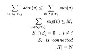
and demand nodes and they must have a total supply greater or equal to its total demand. The total supply in each
of the subgraphs
consists of supply
and demand nodes and they must have a total supply greater or equal to its total demand. The total supply in each
of the subgraphs ![]() must be no more than
a fixed limit
must be no more than
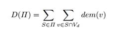
a fixed limit ![]() . The goal is to maximize the fulfillment of demands, or
more precisely to maximize the following sum.
. The goal is to maximize the fulfillment of demands, or
more precisely to maximize the following sum.
Satisfying
the following constraints:
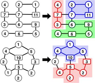
An illustration
of problem instances is given in the following figure:
Problem Instances
We have generated separate sets of problem instances for
general graphs and trees. With the goal of having an extensive set of test
problems a wide range of graph sizes has been considered. The generated test
instances have 10-100 supply nodes and 30-1000 demand nodes. For each pair ![]() ,
number of supply and demand nodes, problem instances having a maximal number of subgraphs
,
number of supply and demand nodes, problem instances having a maximal number of subgraphs ![]() have been generated with the constraint that
have been generated with the constraint that ![]() . For each triplet
. For each triplet ![]() ,
40 different problem instances have been created using different seeds for the
random generator using the following algorithm.
,
40 different problem instances have been created using different seeds for the
random generator using the following algorithm.
The first step was generating ![]() random positive integer numbers, corresponding
to node weights, with a uniform distribution
within the interval [10,39]. General graphs had a total of
random positive integer numbers, corresponding
to node weights, with a uniform distribution
within the interval [10,39]. General graphs had a total of ![]() random edges, with the constraint that
the graph had to be connected. In case
of the second type of graphs, i.e. trees, we would simply generate a random
tree for
random edges, with the constraint that
the graph had to be connected. In case
of the second type of graphs, i.e. trees, we would simply generate a random
tree for ![]() nodes.
nodes.
For both types of graphs, for a problem with a maximal
number of subgraphs ![]() , the next step was to select nsub random nodes
as seeds for the subgraphs (partitions). The subgraphs are grown using an
iterative method until all the nodes of the original graph are contained in one
of the subgraphs. The growth of subgraph
, the next step was to select nsub random nodes
as seeds for the subgraphs (partitions). The subgraphs are grown using an
iterative method until all the nodes of the original graph are contained in one
of the subgraphs. The growth of subgraph
![]() has been performed by expanding it to a random
neighboring node that does not belong to any of the other subgraphs.
has been performed by expanding it to a random
neighboring node that does not belong to any of the other subgraphs.
The number of supply nodes ![]() in each of the subgraph
in each of the subgraph ![]() was
generated using the following iterative procedure. Initially all
was
generated using the following iterative procedure. Initially all ![]() .
At each iteration a random graph
.
At each iteration a random graph ![]() is selected and for it
is selected and for it ![]() is incremented by one if
is incremented by one if ![]() <
|
<
|![]() |-1.
The next step was randomly selecting
|-1.
The next step was randomly selecting ![]() nodes
inside
nodes
inside ![]() which will be supply nodes. The total supply
which will be supply nodes. The total supply ![]() in such partition would be calculated using
the following formula
in such partition would be calculated using
the following formula
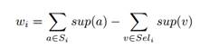
Tehe equation states
that the total supply inside of partition ![]() is equal to the sum of weights of all nodes
inside
is equal to the sum of weights of all nodes
inside ![]() minus
the sum of weights of all the nodes
minus
the sum of weights of all the nodes ![]() selected to be supply nodes. The following
step was distributing the total supply among the nodes that have been selected
to be supply nodes. In practice this means that we randomly generate
selected to be supply nodes. The following
step was distributing the total supply among the nodes that have been selected
to be supply nodes. In practice this means that we randomly generate ![]() numbers having the sum
numbers having the sum ![]() .
This has been done by generating
.
This has been done by generating ![]() distinct random integer numbers between 0 and
distinct random integer numbers between 0 and ![]() .
These numbers are put in an array
.
These numbers are put in an array ![]() with the addition of
with the addition of ![]() and
and ![]() ,
and sorted. The supply corresponding to the i-th node was equal to
,
and sorted. The supply corresponding to the i-th node was equal to ![]() .
The final step was setting the maximal allowed supply in a subgraph
.
The final step was setting the maximal allowed supply in a subgraph ![]() to
the maximal value of
to
the maximal value of ![]() .
.
For problem instances generated using the proposed method
the optimal solution is known and is equal to the sum of supplies of all the
supply nodes. It is important to mention that by using the proposed method for
generating problem instances it is
possible to have partitionings that do not have ![]() subgraphs with demand nodes. This is due to
the possibility that some seed nodes may be cut off from the rest of the graph.
Such partitionings have been excluded
from the test data sets.
subgraphs with demand nodes. This is due to
the possibility that some seed nodes may be cut off from the rest of the graph.
Such partitionings have been excluded
from the test data sets.
The generated test instances have been made available for download.
File Structure
Benchmark data sets are given in one zip file. The file has two folders General, Tree which hold all the problem instances for the specific type of graphs.
In each of these folders there are pairs of “x.gpr” files which give a problem instance definition and “x.sol” which gives the optimal solutions for this instance. The structure of the files is intuitive, but we give the following explanation of the structure
The “gpr” files have the following structure:
“Maximum Number of Subgraphs” % line included for easy reading
NSub
“Maximum Allowed Supply” % line included for easy reading
Ms
“Number of Supply” % line included for easy reading
N % number of supply nodes
“Number of Demmand” % line included for easy reading
M % Number of demand nodes
Weights % line included for easy reading
N+M Lines consisting of one integer value. % Positive means supply node, negative demand node.
Node Ids start from 0
Edges % line included for easy reading
N+M Pairs of lines
Edges(I) % Indicates that edges connected to I will be given next
A line with a list on integers % list of nodes to which node %I% is connected
The “sol” files have
the following structure:
Number Of Partitions ” % line included for easy reading
N % Number of Partitions
N Pairs of lines
SupplyNode I % line included for easy reading, Gives information that I is the supply node
A line with a list of integers % All these nodes are a part of the current partition
The files for on
problem size
For each of the problem sizes there are 40 different problem instances. We have used the following file naming convection:
“test_S_D_N.gpr”, “sol_S_D_I.sol”. Where “S” gives the number of supply nodes, “D” the number of demand nodes, N gives the number of subgraphs and “I” the number of the instance. For example for a graph with 10 supply nodes, and 100 demand nodes, 3 subgraphs, the 15 problem instance files would have the following names
“test_10_100_3_15.gpr”, “sol_10_100_3_15.gpr”.
For each number N of supply nodes we have generated graphs with (N*3, N*5, N*10, N*20) demand nodes.